Science Olympiad Team Generator
An Algorithmic Approach to Automatic Skill Analysis and Team Assignment
1. Introduction
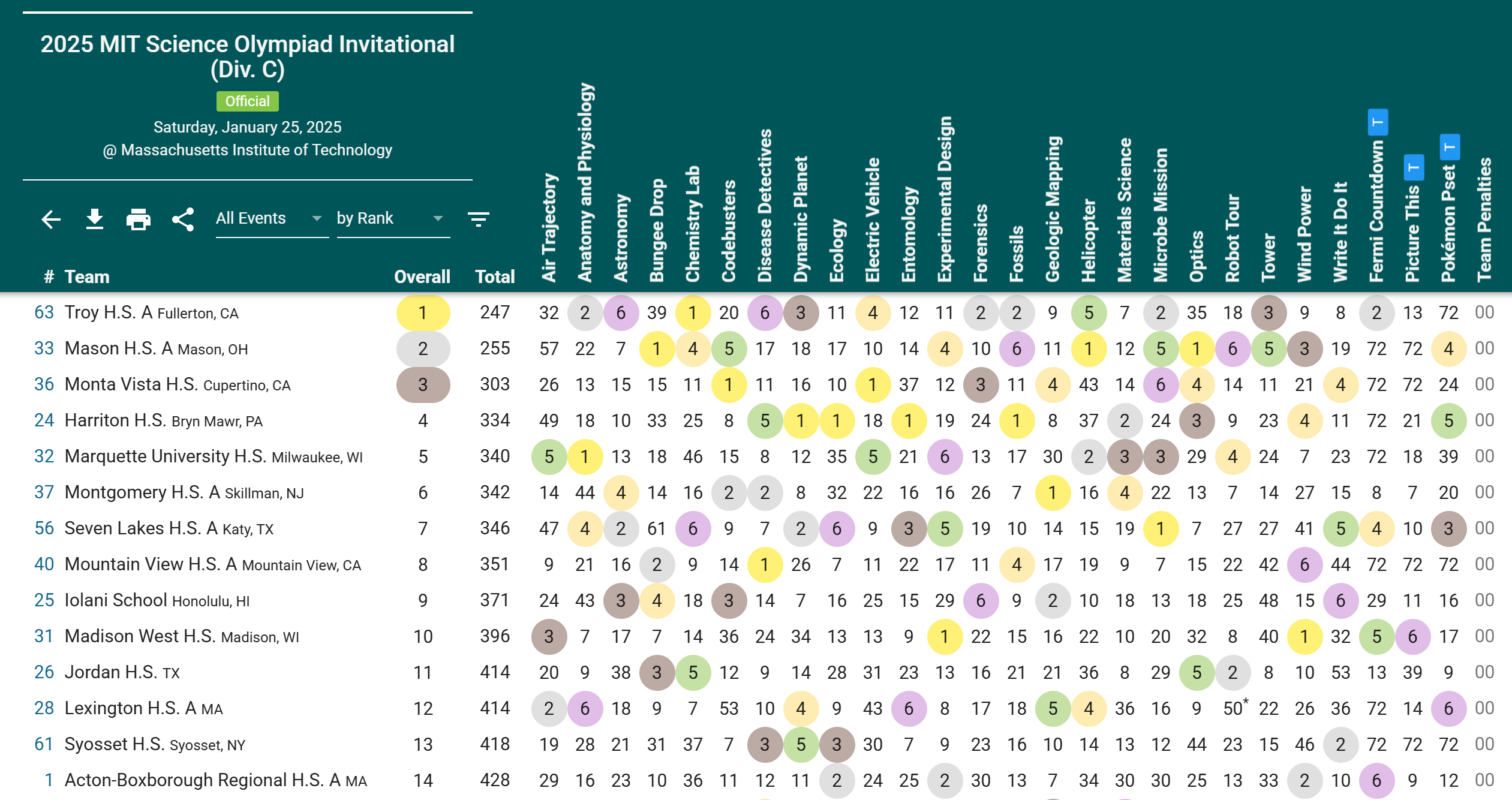
Science Olympiad is a U.S.-based team competition where groups of up to fifteen students compete in various events covering a wide range of scientific and engineering subjects. Competitions usually allow two or three students from the same team to collaborate on any one event, but the number and type of events can differ slightly between competitions. In every event offered at a competition, teams are ranked based on their performance. For example, a team that earns first place in an event has outperformed all other teams in that specific event. If a team does not participate in or cheats on an event, their rank for the event is usually a number higher than the total number of teams competing. Some competitions may also share what specific scores a team gets in an event, though there is often no way to compare results with other teams other than the ranking system.
After a competition ends, each team's overall score is determined by summing their rankings across all events. Teams are then ranked from lowest to highest overall score, with the lowest score indicating the best overall performance. Figure 1 illustrates how competition results are typically displayed, with columns representing events and rows representing teams. Each cell contains the rank that a particular team achieved in a specific event.
To practice for competitions or to evaluate individual skills in particular events, teams might also hold practice tests or tryouts. These involve giving the same individual test to multiple students and comparing the number of points each individual student gains. Those who gain more points than others when taking the same test would be considered better than them in the test's event. Unlike competition data, practice test data provides individual-level performance information rather than team-level rankings.
When creating team assignments for any competition, officers and coaches must focus on two different criteria: skills and preferences. The amount of skill any one member has in an event must be evaluated based on both past competition data and practice test/tryout data. On the other hand, preference data includes both partner preferences and event preferences. Partner preferences refer to a student's preferred partners, whether for a specific event or not, while event preferences indicate the student's preferred events.
Usually, officers and coaches place a higher priority on fulfilling preference requests when creating team assignments for non-qualifier competitions (e.g., invitational competitions), allowing students to explore their interests and find events that they're really passionate about. On the other hand, for qualifying competitions (e.g., Regional, State, and National competitions), officers and coaches prefer team assignments that attempt to maximize performance at a competition. The relative importance of skills versus preferences can vary depending on the competition's significance and the team's goals.
To maximize performance, officers and coaches assign members to events that align best with their areas of expertise. However, determining the best assignments can be challenging because it is difficult to assess individual contributions within collaborative events. Some members may carry most of the workload in an event while their teammate(s) are carried, and results might inflate the carried teammate(s)' individual skill. Other external factors such as luck or the difficulty of the competition can make it challenging to evaluate individual skills and creates an opportunity for biases to influence decisions when creating teams.
Moreover, assessing skills is an extremely time-consuming process, especially when dealing with a large number of students and events. Officers and coaches must carefully assess each student's past performances to ensure that the best members are assigned to the right events. If partner or event preferences are also taken into consideration, complexity increases due to uncertainty on how to properly combine both factors. In addition, many competitions require the submission of team rosters very early before competitions, which often results in rushed decisions that may not fully consider all relevant factors.
Our Contribution: By automating the skill evaluation and team creation processes, fair teams can be created based on preference data and past performance data, minimizing potential for biases and saving valuable time. This document describes the algorithms used to (1) estimate member skills from heterogeneous data sources with varying difficulties, and (2) generate optimal team assignments that balance skill optimization with preference satisfaction.
2. Algorithm Overview
Our approach consists of two main phases. In the first phase, we estimate the skill of each member in each event using historical competition and practice test data. This estimate has several free parameters (difficulty weights and biases for each data source), which we set via leave-one-out cross-validation to ensure our model generalizes well to new competitions.
In the second phase, we use the computed skill estimates along with user-provided preference data to generate team assignments. We define a scoring function that combines skill scores, preference scores, partner bonuses, and required assignment bonuses. We then use a greedy optimization algorithm to construct teams that maximize this score while satisfying various constraints (event capacity, schedule conflicts, senior limits, etc.).
3. Estimating Skills for Members on Events
Before generating optimal teams, there must be a careful analysis of member skill levels in each event. Due to the limited available data, we opted for a simple approach that would ignore partnerships, instead opting for a system based on competition difficulty and experience that can be generalized for all members. The skill estimation process consists of four steps:
- Skill Observations: Convert raw competition ranks and practice test scores into normalized skill observations on a 0-1 scale.
- Skill Adjustments: Apply learned difficulty weights and biases to account for variations in competition/test difficulty.
- Cross-Validation: Use leave-one-out cross-validation to learn optimal difficulty parameters.
- Final Estimates: Compute final skill estimates with experience bonuses and normalization.
3.1 Notation
Throughout this section, we use the following notation:
- \(m\) — a member (student)
- \(e\) — an event
- \(c\) — a competition instance
- \(p\) — a practice test instance
- \(x\) — a generic instance (either competition \(c\) or practice test \(p\))
- \(C\) — the set of all competitions
- \(P\) — the set of all practice tests
- \(X = C \cup P\) — the set of all instances (competitions and practice tests)
- \(X_{me}\) — the subset of instances where member \(m\) participated in event \(e\)
- \(|X_{me}|\) — the number of instances in \(X_{me}\) (i.e., how much experience \(m\) has in event \(e\))
3.2 Step 1: Skill Observations
The first step is to convert raw performance data into normalized skill observations on a common 0-1 scale, where higher values indicate better performance. We process competition ranks and practice test scores differently due to their different nature.
Competition Data
For competitions, we only have access to team-level rankings in each event, not individual scores. If a member participated in an event at a competition, we attribute the team's rank in that event to the member. While this approach cannot distinguish between partners who contributed differently, it provides a reasonable approximation given the available data.
For each member \(m\), event \(e\), and competition \(c\), we define the skill observation as: $$s_{mec} = 1 - \frac{r_{mec} - 1}{N_c - 1}$$ where:
- \(r_{mec}\) is the rank that the team achieved in event \(e\) at competition \(c\) (with member \(m\) participating)
- \(N_c\) is the total number of teams competing at competition \(c\)
This formula maps ranks to a 0-1 scale: a 1st place finish (rank = 1) yields a skill observation of 1, while a last place finish (rank = \(N_c\)) yields a skill observation of 0. For example, if a team placed 3rd out of 50 teams, the skill observation would be \(1 - (3-1)/(50-1) \approx 0.96\).
Practice Test Data
For practice tests and tryouts, we have access to individual scores, which provides more direct measurement of individual skill. For each member \(m\), event \(e\), and practice test \(p\), we define the skill observation as: $$s_{mep} = \frac{g_{mep}}{G_{ep}}$$ where:
- \(g_{mep}\) is the number of points scored by member \(m\) on event \(e\) in practice test \(p\)
- \(G_{ep}\) is the maximum possible points for event \(e\) on practice test \(p\)
This formula directly converts scores to percentages on a 0-1 scale. A member who scored 85 out of 100 points would have a skill observation of 0.85.
Unified Notation
We use \(s_{mex}\) to denote the skill observation for member \(m\) in event \(e\) for any instance \(x\), whether \(x\) is a competition or a practice test. This allows us to treat both data sources uniformly in subsequent steps.
3.3 Step 2: Skill Observation Adjustments
A key challenge in combining data from multiple sources is that different competitions and practice tests have different difficulties. A skill observation of 0.7 from a very difficult invitational should be weighted more heavily than a 0.7 from an easy practice test. Similarly, some data sources might systematically produce higher or lower skill observations due to factors like scoring rubrics or competition format.
To account for these differences, we introduce learnable parameters for each instance. Each competition or practice test \(x\) has two parameters:
- Weight \(w_x\) where \(0 \le w_x \le 1\): Scales the skill observation. A higher weight means performances at this instance are more indicative of true skill (e.g., a harder competition where good performances are more meaningful).
- Bias \(b_x\) where \(-0.5 \le b_x \le 0.5\): Shifts the skill observation. A positive bias might account for a systematically easier competition where everyone scores higher.
The adjusted skill observation is computed as: $$f_{mex} = w_x \cdot s_{mex} + b_x$$
Intuition: Consider two competitions. Competition A is a major invitational with many strong teams, while Competition B is a smaller local competition. We would expect Competition A to have a higher weight (good performances there are more impressive) and possibly a positive bias (even average teams score lower in absolute terms). The cross-validation procedure in the next step will learn appropriate values for these parameters.
3.4 Step 3: Leave-One-Out Cross-Validation
We need to learn the optimal values for the weights \(w_x\), biases \(b_x\), and an initial skill parameter \(a\) (used when a member has no prior experience in an event). We use leave-one-out cross-validation to find parameters that generalize well to predicting performance on held-out instances.
The Cross-Validation Procedure
The key idea is: for each data point we have, can we predict it using the other data points? If a member performed at a certain level in competitions 1, 2, and 3, can we predict their performance in competition 4? The parameters that lead to the best predictions are the ones we want.
-
For each member-event pair \((m, e)\) with instances \(X_{me}\):
We consider each instance \(x_k \in X_{me}\) one at a time and try to predict the skill observation \(s_{mex_k}\) using data from all other instances where this member participated in this event.
-
Computing predictions:
For a held-out instance \(x_k\), we predict the adjusted skill as follows:
- If \(|X_{me}| = 1\) (this is the member's only data point for this event), we use the initial skill parameter: \(\widehat{f_{mex_k}} = a\). This represents a baseline expectation for how a first-timer performs, and a user can choose to disable this parameter if they prefer to exclude single-data-point pairs from the loss.
- Otherwise, we average the adjusted skills from all other instances: $$\widehat{f_{mex_k}} = \frac{1}{|X_{me}| - 1} \sum_{x \in X_{me} \setminus \{x_k\}} f_{mex}$$
We then convert this predicted adjusted skill back to a predicted raw skill observation: $$\widehat{s_{mex_k}} = \frac{\widehat{f_{mex_k}} - b_{x_k}}{w_{x_k}}$$
-
Computing loss per instance:
Let \(\mathcal{P}_{x_k}\) be the set of all member-event pairs \((m, e)\) that have data at instance \(x_k\). The loss for instance \(x_k\) is the mean squared error between actual and predicted skill observations: $$L_{x_k} = \frac{1}{|\mathcal{P}_{x_k}|} \sum_{(m, e) \in \mathcal{P}_{x_k}} (s_{mex_k} - \widehat{s_{mex_k}})^2$$
-
Total loss:
The total loss we minimize is the sum of losses across all instances: $$L = \sum_{x_k \in X} L_{x_k}$$
-
Optimization:
We minimize \(L\) with respect to all parameters \(\{w_x, b_x\}_{x \in X}\) and \(a\) using SciPy's
optimize.minimizefunction with bound constraints. A 5-second time limit is enforced to prevent excessive computation time for large datasets.
Why this works: If a competition is genuinely harder, members who do well there should also do well elsewhere, and vice versa. The cross-validation procedure finds parameters that make these predictions as accurate as possible. Competitions with inconsistent results (perhaps due to unusual conditions) will naturally receive lower weights.
Optional: Disabling the Initial Skill Parameter
Users can choose to disable the initial skill parameter \(a\) via the skill settings. When disabled, member-event pairs with only one data point are excluded from the cross-validation loss entirely, and the optimizer focuses only on pairs with two or more instances. Member-event pairs with no data receive a default skill of 0 instead of \(a\).
Tradeoffs:
- Keep \(a\) enabled (default, recommended when many first-timers): When many members try an event for the first time at different competitions, their results relative to \(a\) provide useful signal for calibrating competition difficulty. First-timers scoring lower at harder competitions and higher at easier ones helps the optimizer learn more accurate weights and biases. The tradeoff is that single-data-point pairs contribute to the loss alongside multi-data-point pairs, and the optimizer must balance fitting both. Since \(a\) is a single shared value that cannot distinguish between strong and weak first-timers, these predictions are inherently less informative—and optimizing them can pull the weights \(w_x\) and biases \(b_x\) away from values that would better fit the more meaningful multi-instance data.
- Disable \(a\) (recommended when most pairs have multiple data points): The optimizer focuses entirely on member-event pairs where cross-validation is most meaningful (2+ instances). This can produce more accurate weights and biases when there is sufficient multi-instance data, since the loss is not diluted by single-data-point predictions that are inherently uninformative. However, this discards the difficulty-calibration signal from first-timers.
3.5 Step 4: Calculating Final Skill Estimates
Using the optimized parameters from Step 3, we compute the skill estimates that will be displayed to users and used for team generation.
-
Handling instances without overlapping data:
Some instances may not share any member-event pairs with other instances. For example, if a practice test was taken only by members who never competed in any of the logged competitions, there's no way to calibrate its difficulty relative to other instances. These instances receive the average weight (\(w_{avg}\)) and bias (\(b_{avg}\)) computed from instances that do have overlapping pairs. If no instances have overlapping pairs (e.g., completely new team with no historical data), we use defaults: \(w_{avg} = 0.5\) and \(b_{avg} = 0\).
-
Computing base skill estimate:
For each member-event pair \((m, e)\) with data, we average all adjusted skill observations: $$\bar{f}_{me} = \frac{1}{|X_{me}|} \sum_{x \in X_{me}} f_{mex}$$ For member-event pairs with no data (member has never participated in this event), we use the initial skill: \(\bar{f}_{me} = a\).
-
Converting to predicted skill:
We convert the average adjusted skill to a predicted skill observation using the average parameters: $$\tilde{s}_{me} = \frac{\bar{f}_{me} - b_{avg}}{w_{avg}}$$ This represents our best estimate of how the member would perform in a "typical" future competition.
-
Adding experience bonus:
Members with more experience in an event receive a bonus to their skill estimate. This serves two purposes: (1) it rewards consistency and dedicated practice, and (2) it prevents members who performed well in only one or two instances from being overrated compared to members with longer track records.
Let \(P\) be a user-specified experience rate parameter, and let \(n_{me} = |X_{me}|\) be the number of instances where member \(m\) participated in event \(e\): $$\tilde{s}'_{me} = \tilde{s}_{me} + P \cdot n_{me}$$
-
Normalizing to [0, 1]:
Finally, we scale all skill estimates to the range [0, 1] for easier interpretation: $$\hat{s}_{me} = \frac{\tilde{s}'_{me} - s_{min}}{s_{max} - s_{min}}$$ where \(s_{min}\) and \(s_{max}\) are the minimum and maximum values of \(\tilde{s}'_{me}\) across all member-event pairs with data.
The final value \(\hat{s}_{me}\) is the skill estimate displayed to the user for member \(m\) in event \(e\). A value of 1.0 indicates the highest-skilled member in that event, while 0.0 indicates the lowest.
4. Generating Teams
With skill estimates computed, we now turn to the problem of generating optimal team assignments. This involves defining constraints that valid team assignments must satisfy, a scoring function that measures assignment quality, and an optimization algorithm to find high-scoring assignments.
4.1 Input Data
In addition to the computed skill estimates, team generation requires several types of user-provided input:
Event Preferences
Coaches and/or officers can optionally provide data on which events each member prefers, ranked from most wanted (rank 1) to least wanted. Figure 2 shows an example of preference data, where each row represents a member and columns show their ranked event preferences. If the "Use Ranked Event Preferences" option is enabled, the ordering matters—higher-ranked events contribute more to the scoring function. If disabled, all listed events are treated equally regardless of order (see Section 4.4.1).

Partner Preferences
Coaches and/or officers can also optionally provide partner preference data, specifying pairs of members who wish to work together on a specific event.
Required Assignments
Sometimes certain members must be assigned to specific events (e.g., a member who has been building a device all season must compete with it). Required member-event pairs can be specified to ensure these constraints are satisfied.
Competition Settings
Additional settings include: the list of events, which events allow 3 members instead of 2, which events are "build events" (with separate limits), schedule conflicts between events, maximum/minimum events per member, maximum build events per member, team size limit, the event preference weight \(w_e\) (see Section 4.4.5), the partner preference weight \(w_p\) (see Section 4.4.5), and whether to use ranked event preferences (see Section 4.4.1).
4.2 Notation
We use the following notation for team generation:
- \(T\) — a team assignment, where \(T_e\) is the set of members assigned to event \(e\)
- \(A_T = \bigcup_{e \in E} T_e\) — the set of unique members on team \(T\)
- \(M\) — set of all available members
- \(E\) — set of all events
- \(E_3 \subseteq E\) — set of events allowing 3 members (instead of the usual 2)
- \(B \subseteq E\) — set of build events
- \(C_e\) — set of events that conflict with event \(e\) (cannot be done by the same member due to schedule overlap)
- \(o_M\) — maximum team size (number of unique members)
- \(o_\Gamma\) — maximum events per member
- \(o_\gamma\) — minimum events per member
- \(o_B\) — maximum build events per member
- \(w_e\) — event preference weight parameter (controls how much event preferences influence team score)
- \(w_p\) — partner preference weight parameter (controls how much partner preferences influence team score)
- \(r\) — randomization parameter (controls the magnitude of random noise added to skill scores, range \([0, 1]\))
- \(d\) — the maximum number of preferences any member listed
- \(p_{me}\) — preference rank of event \(e\) for member \(m\) (1 = top choice; if not listed, \(p_{me} = d + 1\))
- \(\hat{s}_{me}\) — skill estimate for member \(m\) in event \(e\) (from Section 3)
- \(q_m\) — binary indicator: 1 if member \(m\) is a senior, 0 otherwise
4.3 Step 1: Team Validity Constraints
Not all team assignments are valid. A valid assignment must satisfy several constraints related to event capacity, member limits, schedule conflicts, and Science Olympiad rules. We define a function \(v(T, m, e)\) that returns True if adding member \(m\) to event \(e\) on team \(T\) would result in a valid assignment.
All of the following constraints must be satisfied for \(v(T, m, e) = \text{True}\):
-
Event Capacity:
Each event has a maximum number of participants (usually 2, sometimes 3). The event must have room for another member:
\[ |T_e| < \begin{cases} 3 & \text{if } e \in E_3 \text{ (events allowing 3 members)} \\ 2 & \text{otherwise} \end{cases} \] -
No Duplicate Assignment:
A member cannot be assigned to the same event twice:
\[m \notin T_e\] -
Maximum Events per Member:
Each member can only participate in up to \(o_\Gamma\) events total:
\[|\{e' \in E : m \in T_{e'}\}| < o_{\Gamma}\] -
Maximum Build Events per Member:
Build events require significant preparation time. If \(e\) is a build event, the member must not have reached their build event limit:
\[e \in B \Rightarrow |\{e' \in B : m \in T_{e'}\}| < o_B\] -
No Schedule Conflicts:
Some events occur at the same time during competition. A member cannot be assigned to events that conflict:
\[\forall e' \in C_e: m \notin T_{e'}\] -
Team Size Limit:
The total number of unique members on the team cannot exceed \(o_M\) (typically 15):
\[m \in A_T \text{ or } |A_T| < o_M\](If the member is already on the team, this constraint is automatically satisfied.)
-
Senior Limit:
Science Olympiad rules limit the number of seniors (12th graders) to 7 per team:
\[(q_m = 0) \text{ or } (m \in A_T) \text{ or } |\{m' \in A_T : q_{m'} = 1\}| < 7\](Non-seniors can always be added. Seniors already on the team can be assigned to more events. New seniors can only be added if there are fewer than 7 seniors currently.)
Validity Check: The function \(v(T, m, e) = \text{True}\) if and only if all seven constraints above are satisfied.
4.4 Step 2: Team Scoring Function
We define a scoring function \(h(T)\) that measures how good a team assignment is. Higher scores are better. The score combines four components: event preference satisfaction, skill optimization, partner preference satisfaction, and required assignment fulfillment.
4.4.1 Event Preference Score \(h_P(T)\)
Members should be assigned to events they prefer. Higher-ranked preferences contribute more to the score, normalized so that each member's total possible preference contribution sums to 1: $$h_P(T) = \sum_{e \in E} \sum_{m \in T_e} \begin{cases} \frac{2(d - p_{me} + 1)}{d(d + 1)} & \text{if member } m \text{ listed event } e \text{ as a preference} \\ 0 & \text{otherwise} \end{cases}$$
Explanation: The denominator \(\frac{d(d+1)}{2}\) is the sum \(d + (d-1) + \cdots + 1\), ensuring that if a member is assigned to all \(d\) of their listed preferences, their total contribution is exactly 1. For example, if a member listed 5 preferences (so \(d = 5\)) and is assigned to their 1st choice, they contribute \(\frac{2 \cdot 5}{5 \cdot 6} = \frac{1}{3} \approx 0.33\). Their 2nd choice would contribute \(\frac{2 \cdot 4}{30} \approx 0.27\), and so on. Events not listed as preferences contribute 0.
Optional: Use Ranking
The "Use Ranked Event Preferences" option controls whether the order of a member's event preferences matters when computing the preference score.
- Enabled (default): Higher-ranked preferences contribute more to the score, as shown in the formula above, but normalized so that all preferences sum to 1. A member's 1st choice is worth more than their 2nd, which is worth more than their 3rd, etc. This is useful when members have a clear ordering of which events they care about most.
- Disabled: All listed preferences count equally as \(\frac{1}{d}\), regardless of the order they were listed. The algorithm only cares whether an event was listed as a preference, not where it was ranked. This is useful when members list events they'd be happy doing without a strong ordering preference.
4.4.2 Skill Score \(h_S(T)\)
The team should include skilled members in each event. The skill score is simply the sum of skill estimates for all assigned member-event pairs: $$h_S(T) = \sum_{e \in E} \sum_{m \in T_e} \hat{s}_{me}$$
This encourages assigning members to events where they have demonstrated strong past performance.
4.4.3 Partner Preference Bonus \(h_M(T)\)
Some members want to work with specific partners on specific events. Let \(Y\) be the set of partner preference pairs \((m_1, m_2, e)\), indicating that members \(m_1\) and \(m_2\) want to be partners on event \(e\).
The partner preference bonus is the fraction of satisfied partner requests: $$h_M(T) = \frac{1}{|Y|} \sum_{(m_1, m_2, e) \in Y} \mathbb{1}\big[\{m_1, m_2\} \subseteq T_e\big]$$
Key design choices:
- Event-specific only: Each partner request specifies a particular event, so each request is either satisfied (both members on that event) or not. This avoids the issue of general partner preferences incentivizing the algorithm to assign both members to as many shared events as possible.
- Normalization by \(|Y|\): Dividing by the total number of partner requests ensures \(h_M(T) \in [0, 1]\), keeping it on a comparable scale to other scoring components.
4.4.4 Required Assignment Bonus \(h_K(T)\)
Some member-event assignments are required and must be fulfilled. Let \(K\) be the set of required member-event pairs \((m, e)\): $$h_K(T) = 10000 \cdot |\{(m,e) \in K : m \in T_e\}|$$
The large multiplier (10000) ensures that required assignments are effectively treated as hard constraints—any team that fails to satisfy them will score much lower than teams that do.
4.4.5 Final Team Score
The final score combines all components. The skill score serves as the baseline, with event preferences and partner preferences added on top via user-specified weights: $$h(T) = h_S(T) + w_e \cdot h_P(T) + w_p \cdot h_M(T) + h_K(T)$$
The parameter \(w_e \ge 0\) controls how much event preferences influence the team score relative to skill:
- \(w_e = 0\): Optimize purely for skill (ignore event preferences)
- \(w_e = 0.5\): Event preferences have moderate influence alongside skill
- \(w_e = 1\): Event preferences are weighted equally with skill
The parameter \(w_p \ge 0\) controls how much partner preferences influence the team score. A small value (e.g., \(w_p = 0.05\)) makes partner preferences act as a tiebreaker between otherwise similar assignments, while a larger value gives them more influence. Setting \(w_p = 0\) disables partner preferences entirely.
For important qualifying competitions, coaches might set \(w_e\) and \(w_p\) low to prioritize skill. For invitational competitions focused on development, higher values of \(w_e\) and \(w_p\) give more weight to member satisfaction.
4.4.6 Randomization
The algorithm is deterministic by default—running it twice with the same inputs produces the same team. While this is desirable for reproducibility, it means the algorithm always converges to the same local optimum found by the greedy search. The randomization parameter \(r \in [0, 1]\) introduces controlled noise into the skill scores, allowing the algorithm to explore different assignments.
When \(r > 0\), the skill score is modified by adding a small random perturbation to each member-event skill estimate: $$h_S(T) = \sum_{e \in E} \sum_{m \in T_e} \big(\hat{s}_{me} + \epsilon_{me}\big)$$ where \(\epsilon_{me} = \big(R(m, e) - 0.5\big) \cdot r\) and \(R(m, e) \in [0, 1)\) is a pseudorandom value.
The noise term \(\epsilon_{me}\) is uniformly distributed in \(\big[-\frac{r}{2}, \frac{r}{2}\big)\). At \(r = 0\), no noise is added and the algorithm behaves as before. At \(r = 1\), the noise can shift each skill estimate by up to \(\pm 0.5\), which is enough to occasionally change assignment decisions when members have similar skill levels.
Seeded randomness: The random value \(R(m, e)\) is generated using a seeded pseudorandom number generator (PRNG) keyed on the member-event pair. Specifically, a hash is computed from the concatenation of the member's name and the event's name, and this hash is used as the seed for a Mulberry32 PRNG. This means:
- The same member-event pair always receives the same random perturbation, so regenerating with the same settings produces the same result.
- Different member-event pairs receive different (uncorrelated) perturbations.
- To get a genuinely different team assignment, the coach must change some input (e.g., a member name, event name, or other setting), which changes the hash seeds and produces new perturbations.
When to use randomization: Randomization is most useful when the algorithm produces a team that seems suboptimal due to greedy decisions. A small amount of randomization (e.g., \(r = 0.1\)) can nudge the algorithm into exploring slightly different paths during the greedy search, potentially finding a better local optimum. Larger values (e.g., \(r = 0.5\) or higher) introduce more variability and may produce significantly different team compositions, which can be useful for exploring alternative team structures.
4.5 Step 3: Greedy Team Construction
Finding the globally optimal team assignment is computationally intractable for realistic problem sizes. With \(n\) members, \(e\) events, and teams of size \(k\), the number of possible team assignments grows combinatorially—even a modest scenario with 30 members, 23 events, and teams of 15 would have billions of possible configurations. This makes exhaustive search infeasible.
Instead, we use a greedy algorithm that builds teams incrementally by making locally optimal decisions at each step. The greedy approach works as follows: rather than considering all possible complete teams at once, we build the team one member at a time, always choosing the member (and their event assignments) that most improves the team score at that moment. While this doesn't guarantee finding the globally optimal solution, it produces good solutions efficiently and has several practical advantages:
- Efficiency: The algorithm runs in polynomial time, making it practical for real-world use.
- Interpretability: Each decision can be explained (e.g., "Alice was added because she has strong skills in Chemistry and listed it as her top preference").
- Flexibility: The algorithm naturally handles constraints and can be easily modified.
The algorithm consists of three main procedures, which we describe in detail below with pseudocode. Understanding how these procedures interact is key to understanding the overall team generation process.
4.5.1 Find Optimal Event Addition: \(j_E(T, m, \text{necessary})\)
This is the most fundamental building block of our algorithm. Given a team \(T\) and a member \(m\) who needs to be assigned to more events, this function finds the single best event to assign \(m\) to. It answers the question: "Given the current state of the team, what's the best event we can add this member to?"
The necessary parameter is crucial and controls the algorithm's behavior:
- When
necessary = True: We must find an assignment for this member, even if it temporarily decreases the team score. This is used when we're trying to meet the minimum events requirement for a member—we can't just skip them because no assignment improves the score. - When
necessary = False: We only accept assignments that improve (or at least don't decrease) the team score. This is used when assigning optional additional events beyond the minimum.
Inputs
- \(T\): Current team assignment (a mapping from events to sets of members)
- \(m\): The member we want to assign to an event
- \(\text{necessary}\): Boolean flag—if True, we must find an assignment even if score decreases
Output
An updated team \(T^*\) with \(m\) assigned to one additional event, or null if no valid assignment exists.
Pseudocode
function FindOptimalEventAddition(T, m, necessary):
    best_team ← null
    best_score_delta ← -∞
    original_score ← h(T)

    for each event e ∈ E do
        if m ∉ T_e then  // member not already on this event

            // Case 1: Direct addition is valid
            if v(T, m, e) = True then
                T' ← copy(T)
                T'_e ← T'_e ∪ {m}
                Δh ← h(T') - original_score

                if Δh > best_score_delta then
                    best_team ← T'
                    best_score_delta ← Δh

            // Case 2: Try replacing existing members
            else
                for each member m' ∈ T_e, m' ≠ m do
                    events_by_m' ← |{e' ∈ E : m' ∈ T_e'}|

                    // Can only replace if m' has extra events and isn't required
                    if events_by_m' > o_γ and (m', e) ∉ K then
                        T' ← copy(T)
                        T'_e ← T'_e \ {m'}  // remove m'

                        if v(T', m, e) = True then
                            T'_e ← T'_e ∪ {m}  // add m
                            Δh ← h(T') - original_score

                            // Accept if necessary OR if score improves
                            if (necessary or Δh ≥ 0) and Δh > best_score_delta then
                                best_team ← T'
                                best_score_delta ← Δh

    return best_team
Detailed Explanation
The function iterates through every event in \(E\) and considers two cases for each:
Case 1: Direct Addition
First, we check if we can simply add \(m\) to event \(e\) without removing anyone. This is possible when all validity constraints are satisfied (the event has capacity, \(m\) hasn't reached their event limit, there are no schedule conflicts, etc.). If valid, we:
- Create a copy of the current team \(T'\)
- Add member \(m\) to event \(e\) in the copy
- Calculate how much this changes the team score: \(\Delta h = h(T') - h(T)\)
- If this is the best improvement we've seen so far, remember this configuration
Case 2: Replacement
If direct addition is not valid (typically because the event already has the maximum number of members), we consider replacing an existing member on that event. For each member \(m'\) currently assigned to event \(e\), we check if replacement is allowed:
- Minimum events check: Member \(m'\) must have more than \(o_\gamma\) events currently assigned. If they're at exactly the minimum, removing them from this event would violate constraints, so we can't replace them.
- Required assignment check: The pair \((m', e)\) must not be in the required assignments set \(K\). If a coach specifically required \(m'\) to be on event \(e\), we can't remove them.
- Score improvement check: If
necessary = False, the replacement must improve the score (\(\Delta h \ge 0\)). Ifnecessary = True, we accept the replacement even if the score decreases (because we must place \(m\) somewhere).
Why Replacement Matters
Consider this scenario: Alice is highly skilled in Chemistry, but the Chemistry event is already full with Bob and Carol. Without the replacement mechanism, Alice couldn't be assigned to Chemistry at all. But suppose Bob is mediocre at Chemistry and has 5 other events (well above the minimum). The replacement logic allows us to remove Bob from Chemistry and add Alice, improving the team's overall Chemistry performance. Bob still has his other events, so no constraints are violated.
Return Value
The function returns the team configuration that achieves the best score improvement (or least score decrease, if necessary = True). If no valid assignment exists at all—perhaps due to schedule conflicts or the member already being on all possible events—it returns null.
4.5.2 Find Optimal Member Addition: \(j_M(T, M_{\text{pool}})\)
While the previous function finds the best event for a given member, this function finds the best member to add to the team from a pool of candidates. It simulates adding each candidate with their optimal event assignments and returns the candidate that results in the highest team score.
This function is the key decision-maker in team construction: at each step, it determines which member should be added next. The answer depends not just on individual skill, but on how well each candidate complements the existing team.
Inputs
- \(T\): Current team assignment
- \(M_{\text{pool}}\): Set of candidate members to consider (might be required members, or all available members)
Output
A tuple containing (1) the updated team \(T^\#\) with the best member added and assigned to events, and (2) the member \(m^*\) who was added. Returns null if no candidate can be validly added.
Pseudocode
function FindOptimalMemberAddition(T, M_pool):
    best_team ← null
    best_member ← null
    best_score ← -∞
    A_T ← {m : m ∈ T_e for some e ∈ E}  // members already on team

    for each member m ∈ M_pool \ A_T do  // candidates not on team
        T_working ← copy(T)
        success ← True

        // Phase 1: Assign minimum required events (must succeed)
        for i ← 1 to o_γ do
            T_result ← FindOptimalEventAddition(T_working, m, necessary=True)
            if T_result = null then
                success ← False
                break
            T_working ← T_result

        // Phase 2: Assign additional events if beneficial (optional)
        if success then
            for i ← 1 to (o_Γ - o_γ) do
                T_result ← FindOptimalEventAddition(T_working, m, necessary=False)
                if T_result ≠ null then
                    T_working ← T_result
                else
                    break  // no more beneficial additions

            // Evaluate this candidate
            score ← h(T_working)
            if score > best_score then
                best_team ← T_working
                best_member ← m
                best_score ← score

    return (best_team, best_member)
Detailed Explanation
For each candidate member \(m\) who isn't already on the team, the algorithm simulates what the team would look like if we added them:
Phase 1: Minimum Events (Mandatory)
Every member on a Science Olympiad team must participate in at least \(o_\gamma\) events (often 1-2). In this phase, we call FindOptimalEventAddition exactly \(o_\gamma\) times with necessary=True. This ensures we find assignments even if they don't immediately improve the score.
If we cannot find \(o_\gamma\) valid event assignments for this candidate (perhaps due to schedule conflicts or other constraints), we mark them as unsuccessful and move on to the next candidate. This prevents us from adding members who would violate the minimum events requirement.
Phase 2: Additional Events (Optional)
After satisfying the minimum, we try to assign additional events up to the maximum \(o_\Gamma\). However, these assignments are only made if they improve (or maintain) the team score (necessary=False). This reflects the reality that:
- Some members are versatile and can effectively contribute to many events
- Other members are specialists who should focus on their strengths
- Assigning a member to an event they're weak in might hurt the team more than help
We stop adding events as soon as no beneficial assignment can be found. For example, if a member is excellent at Chemistry and Biology but weak at everything else, they might end up with just 2 events even if the maximum is 5.
Evaluation
After simulating the addition of candidate \(m\), we compute the total team score \(h(T_{\text{working}})\). We track the candidate who achieves the highest score. Note that we're comparing final team scores, not just the score improvement from adding this member—this ensures we make globally good decisions.
Why This Two-Phase Approach?
Consider Alice and Bob, both candidates for the team. Alice is moderately good at many events, while Bob is exceptional at one event but weak at others. With a minimum of 2 events:
- Alice might get assigned to Events A, B, C, D (all beneficial)
- Bob might get assigned to Event X (excellent) and Event Y (forced, because he needs 2 events minimum)
The two-phase approach ensures Bob gets his strong event assignment, but doesn't force him into multiple weak events. The final comparison picks whichever candidate (with their full assignment) results in a better team.
4.5.3 Build Team: \(\text{make_team}()\)
This is the main orchestrating function that constructs a complete team by repeatedly calling the helper functions above. It handles the overall flow: first adding required members, then filling remaining spots with the best available candidates, and finally ensuring all events have participants.
Inputs
- \(M\): Set of all available members
- \(\mathcal{R}\): Set of required members who must be on this team (e.g., team captains, members with required assignments)
- \(K\): Set of required member-event pairs (e.g., "Alice must do Chemistry")
- \(o_M\): Maximum team size (typically 15 for Science Olympiad)
Output
A complete team assignment \(T\) mapping every event to its assigned members.
Pseudocode
function MakeTeam(M, R, K, o_M):
    // Initialize empty team
    T ← {e ↦ ∅ : e ∈ E}  // all events have empty member sets
    team_members ← ∅

    // Phase 1: Add all required members first
    while |team_members| < |R| do
        (T_new, m_new) ← FindOptimalMemberAddition(T, R)
        if T_new = null then
            break  // cannot add more required members
        T ← T_new
        team_members ← team_members ∪ {m_new}

    // Phase 2: Fill remaining spots with best available members
    while |team_members| < o_M do
        // Exclude members required on other teams
        candidates ← M \ (members required on other teams)
        (T_new, m_new) ← FindOptimalMemberAddition(T, candidates)
        if T_new = null then
            break  // cannot add more members
        T ← T_new
        team_members ← team_members ∪ {m_new}

    // Phase 3: Fix any empty events
    T ← FixEmptyEvents(T, team_members)

    return T
Detailed Explanation
Initialization:
We start with a completely empty team—every event has no members assigned. We also maintain a set team_members to track who has been added so far.
Phase 1: Required Members
Some members must be on the team regardless of their skill scores. This includes:
- Members with required assignments in \(K\) (e.g., someone who built a device all season must compete with it)
- Members explicitly marked as required by the coach (e.g., team captains)
We add required members first because they must be on the team—it would be incorrect to fill all spots with "optimal" members and then have no room for required ones. By processing them first, we ensure they're included and can then optimize the remaining spots around them.
Even among required members, we use FindOptimalMemberAddition to determine the best order to add them and their optimal event assignments. This matters because the order affects which events are available for later members.
Phase 2: Filling Remaining Spots
After required members are placed, we fill the remaining spots (up to the team size limit \(o_M\)) with the best available candidates. At each step, FindOptimalMemberAddition considers all candidates and selects the one who would most improve the team.
This is where the greedy algorithm makes its key decisions. The first few members added often have many good event options, while later members must work around existing assignments. The algorithm naturally handles this by always choosing the currently best option.
Note that we exclude members who are required on other teams from consideration. This is important when generating multiple teams (see below)—we don't want to accidentally place someone on Team 1 when they're supposed to be on Team 2.
Phase 3: Fixing Empty Events
After adding all members, some events might still be empty. This typically happens with:
- New events that no member has experience in or preferences for
- Unpopular events that no one listed as a preference
- Events with many schedule conflicts
The FixEmptyEvents function (described below) addresses this by assigning existing team members to unfilled events.
4.5.4 Fix Empty Events
After the main team construction phases, some events may still lack participants. In Science Olympiad, every event typically needs to be filled—leaving an event empty means the team earns no points there, which significantly hurts overall placement. This helper function ensures all events have at least some coverage.
Why Events Might Be Empty
- New events: Science Olympiad rotates events periodically. A brand-new event has no historical performance data, so members have skill estimates of \(a\) (the default), and may not have listed it as a preference.
- Unpopular events: Some events are consistently unpopular (perhaps perceived as boring or difficult). If no one lists them as preferences, the algorithm might not assign anyone during normal team construction.
- Schedule conflicts: Events that conflict with many popular events might get left empty because members who might have done them are already committed elsewhere.
Pseudocode
function FixEmptyEvents(T, team_members):
    // Count empty spots across all events
    empty_spots ← Σ_{e ∈ E} (capacity(e) - |T_e|)

    while empty_spots > 0 do
        best_team ← null
        best_score ← -∞

        // Try all valid (event, member) assignments
        for each event e ∈ E do
            for each member m ∈ team_members do
                if v(T, m, e) = True then
                    T' ← copy(T)
                    T'_e ← T'_e ∪ {m}
                    score ← h(T')

                    if score > best_score then
                        best_team ← T'
                        best_score ← score

        if best_team ≠ null then
            T ← best_team
            empty_spots ← empty_spots - 1
        else
            break  // no more valid assignments possible

    return T
Detailed Explanation
This function takes a simpler approach than the main construction algorithms. Rather than considering complex replacements, it just looks at all valid (event, member) pairs and greedily selects the one that maximizes the team score.
For each empty spot, the algorithm:
- Iterates through all events \(e\) that have room for more members
- For each event, considers every team member \(m\) who isn't already on that event
- Checks if adding \(m\) to \(e\) is valid (considering schedule conflicts, event limits, etc.)
- If valid, computes the team score that would result
- Selects the assignment that achieves the highest score
This process repeats until all events are filled or no more valid assignments exist. In practice, some events might remain unfilled if no team member can be validly assigned (e.g., if all members have schedule conflicts with that event).
Why This Phase Is Needed
One might wonder why events can still be empty after the main greedy construction, given that each member is assigned up to \(o_\Gamma\) events. The key reason is that replacements during later steps can retroactively free up spots. The main loop processes members sequentially: when member \(m_1\) is added at step 3 and assigned to 4 events (unable to reach 5 due to schedule conflicts), the algorithm moves on. Later at step 8, member \(m_2\) might replace someone on Event X via the replacement mechanism, freeing an open slot on Event X. Member \(m_1\) could now validly fill that slot, but the main loop has already moved past them. This phase catches those cases by re-scanning all team members against all events after the full team is assembled.
Note on Optimality
This greedy approach doesn't guarantee optimal filling of empty events. A more sophisticated algorithm might recognize that moving Alice from Event A to Event B, and then assigning Bob to Event A, produces a better overall result. However, the simple greedy approach works well in practice because most "leftover" events are genuinely less important to the team's success.
4.5.5 Generating Multiple Teams
Many schools need to generate multiple teams for a competition. For example, a large school might have both a Varsity team (competing for placement) and a Junior Varsity team (for development and experience). The algorithm handles this by generating teams sequentially, with earlier teams getting priority.
Pseudocode
function GenerateAllTeams(teams_config, M, all_required_members):
    generated_teams ← []
    available_members ← M

    for t ← 1 to |teams_config| do
        R_t ← required members for team t
        K_t ← required member-event pairs for team t
        o_M_t ← team size for team t

        // Generate this team
        (T_t, members_t) ← MakeTeam(available_members, R_t, K_t, o_M_t)
        generated_teams.append(T_t)

        // Remove assigned members from pool
        available_members ← available_members \ members_t

    return generated_teams
Detailed Explanation
The key insight is that teams are generated sequentially, not simultaneously. This has important implications:
Sequential Generation:
Teams are generated in the order they appear in the configuration. The first team gets first pick of all available members. Once Team 1 is complete, its members are removed from the pool, and Team 2 is generated from the remaining members. This continues for all teams.
Priority Implications:
The ordering of teams matters significantly. If Varsity is generated first, it will get the strongest members based on skill and preference scores. JV will then be optimized from whoever remains. Coaches should order teams by priority—typically Varsity first, then JV, then additional teams.
Required Members Across Teams:
Each team has its own set of required members \(R_t\). A member who is required on Team 2 will be automatically excluded from Team 1's candidate pool, ensuring they're available when Team 2 is generated. This allows coaches to control team composition across multiple teams.
Fairness Considerations:
While this sequential approach is simple and efficient, it's worth noting that it optimizes each team independently rather than jointly optimizing all teams together. In some cases, a different distribution of members might make both teams stronger overall. However, joint optimization would be computationally much more expensive, and the sequential approach aligns with how coaches typically think about team priority.
Example:
Suppose a school has 25 members and needs to create a 15-person Varsity team and a 10-person JV team:
- Varsity is generated first, selecting the 15 members who produce the highest team score
- These 15 members are removed from the pool
- JV is generated from the remaining 10 members (who are automatically all selected since that equals the JV team size)
If some members are required on JV (perhaps younger students who need development experience), they would be excluded from Varsity consideration even in step 1.
5. Limitations and Future Work
While this algorithm provides a systematic and fair approach to team generation, several limitations should be noted:
- Partnership effects: The current skill estimation ignores the effect of partnerships. A member might perform very differently depending on their partner, but we cannot distinguish this from the available data.
- Greedy optimization: The team generation algorithm is greedy and does not guarantee globally optimal solutions. More sophisticated optimization techniques (e.g., simulated annealing, genetic algorithms) could potentially find better solutions.
- Cold start problem: New members with no historical data receive the initial skill estimate \(a\), which may not accurately reflect their abilities.
- Event difficulty variation: The algorithm assumes consistent event difficulty across competitions, but some events may be harder at certain competitions than others.
Future improvements could include modeling partnership effects, using more sophisticated optimization algorithms, and incorporating additional data sources such as practice test performance trends over time.
If you have ideas on how to improve the algorithm, please contact us!